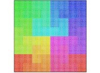
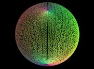
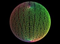
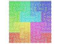
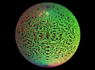
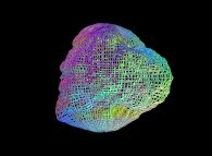
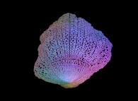
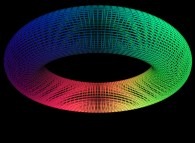
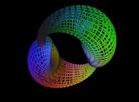
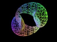
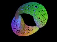
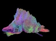
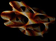
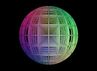
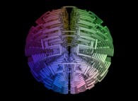
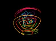
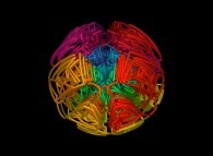
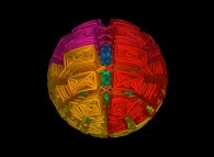
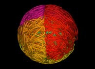
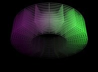
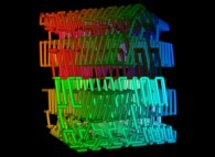
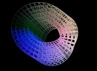
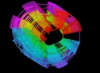
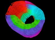
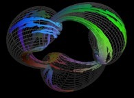
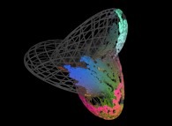
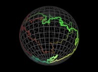
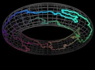
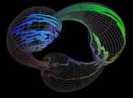
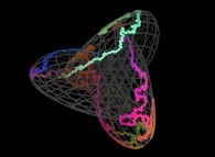
Hilbert and Peano Space filling Curves and Beyond:
From Squares and Cubes to Surfaces (bidimensional Manifolds) and tridimensional Manifolds
CMAP (Centre de Mathématiques APpliquées) UMR CNRS 7641, École polytechnique, Institut Polytechnique de Paris, CNRS, France
[Site Map, Help and Search [Plan du Site, Aide et Recherche]]
[The Y2K Bug [Le bug de l'an 2000]]
[Real Numbers don't exist in Computers and Floating Point Computations aren't safe. [Les Nombres Réels n'existent pas dans les Ordinateurs et les Calculs Flottants ne sont pas sûrs.]]
[Please, visit A Virtual Machine for Exploring Space-Time and Beyond, the place where you can find more than 10.000 pictures and animations between Art and Science]
(CMAP28 WWW site: this page was created on 01/03/2023 and last updated on 01/24/2025 18:15:22 -CET-)
[en français/in french]
Contents:
1-The bidimensional Peano Surjection:
Giuseppe Peano defined the following surjection
:
[0,1] --> [0,1]x[0,1]
Let's T being a real number defined using the base 3
:
T = 0.A1A2A3... ∈ [0,1] with Ai ∈ {0,1,2}
Let's X(T) and Y(T) being two real functions of T defined as
:
X(T) = 0.B1B2B3... ∈ [0,1] with Bi ∈ {0,1,2}
Y(T) = 0.C1C2C3... ∈ [0,1] with Ci ∈ {0,1,2}
with
:
Bn = A2n-1 if A2+A4+...+A2n-0 is even
Bn = 2-A2n-1 otherwise
Cn = A2n if A1+A3+...+A2n-1 is even
Cn = 2-A2n otherwise
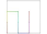
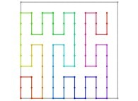
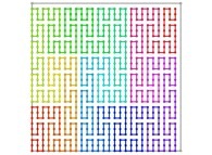
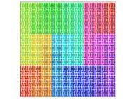
These two functions X(T) and Y(T) are the coordinates of a point P(T) inside the [0,1]x[0,1] square.
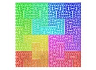
The displayed "curve" -as little spheres- is the trajectory of P(T) when T varies from 0 (lower left corner) to 1-epsilon (upper right corner).
Here are the four first bidimensional Peano curves with an increasing number of digits
{2,4,6,8}:
 [See the used color set to display the parameter T]
2-The tridimensional Peano Surjection:
A tridimensional surjection can be defined
:
[0,1] --> [0,1]x[0,1]x[0,1]
as a generalization of the bidimensional one.
Let's T being a real number defined using the base 3
:
T = 0.A1A2A3... ∈ [0,1] with Ai ∈ {0,1,2}
Let's X(T), Y(T) and Z(T) being three real functions of T defined as:
X(T) = 0.B1B2B3... ∈ [0,1] with Bi ∈ {0,1,2}
Y(T) = 0.C1C2C3... ∈ [0,1] with Ci ∈ {0,1,2}
Y(T) = 0.D1D2D3... ∈ [0,1] with Di ∈ {0,1,2}
with
:
Bn = A3n-2 if A3+A6+...+A3n-0 is even
Bn = 2-A3n-2 otherwise
Cn = A3n-1 if A2+A5+...+A3n-1 is even
Cn = 2-A3n-1 otherwise
Dn = A3n if A1+A4+...+A3n-2 is even
Dn = 2-A3n otherwise
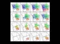
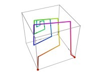
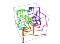
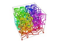
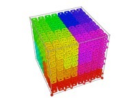
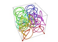
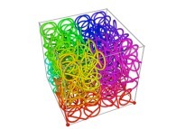
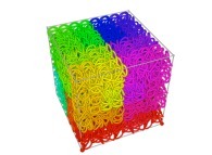
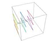
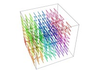
These three functions X(T), Y(T) and Z(T) are the coordinates of a point P(T) inside the [0,1]x[0,1]x[0,1] cube.
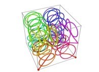
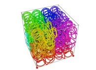
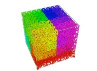
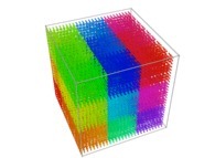
The displayed "curve" is the trajectory of P(T) -displayed as little spheres- when T varies from 0 (lower left corner) to 1-epsilon (upper right corner).
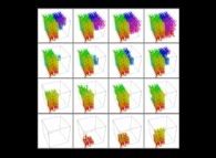
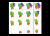
Here are the three first tridimensional Peano curves with an increasing number of digits
{3,6,9}:
 [See the used color set to display the parameter T]
3-The bidimensional Hilbert Curves:
Let's C1(T) being
a parametric curve
defined by means of 2 real functions of T
(T ∈ [0,1])
X1(T) ∈ [0,1] and Y1(T) ∈ [0,1]
such as
:
X1(T=0)=0 Y1(T=0)=0 (lower left corner)
X1(T=1)=1 Y1(T=1)=0 (lower right corner)
Then one defines a sequence of curves Ci(T) (i >= 1) as follows
:
Ci(T) = {Xi(T),Yi(T)} ∈ [0,1]x[0,1] --> Ci+1(T) = {Xi+1(T),Yi+1(T)} ∈ [0,1]x[0,1]
                    if T ∈ [0,1/4[:
                              Xi+1(T) =   Yi(4T-0)
                              Yi+1(T) =   Xi(4T-0)
                                                   Transformation 1
                    if T ∈ [1/4,2/4[:
                              Xi+1(T) =   Xi(4T-1)
                              Yi+1(T) = 1+Yi(4T-1)
                                                   Transformation 2
                    if T ∈ [2/4,3/4[:
                              Xi+1(T) = 1+Xi(4T-2)
                              Yi+1(T) = 1+Yi(4T-2)
                                                   Transformation 3
                    if T ∈ [3/4,1]:
                              Xi+1(T) = 2-Yi(4T-3)
                              Yi+1(T) = 1-Xi(4T-3)
                                                   Transformation 4
Please note that 4=2d where d=2 is the space dimension.
See a special C1(T) curve 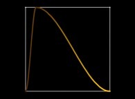 in order to understand the geometrical meaning of the 4 transformations
 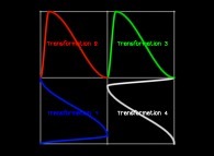 and of their order
 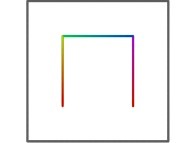 .
.
Here are the five first bidimensional Hilbert curves with an increasing number of iterations
:

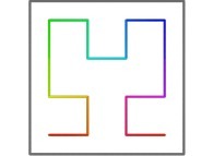
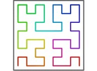
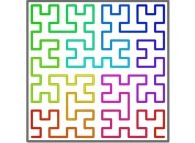
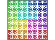 [See the used color set to display the parameter T]
See the construction of some of them
:



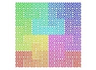
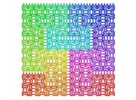
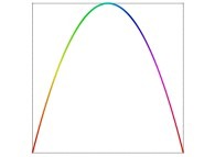
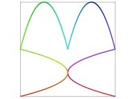
Here are some examples of Hilbert-like bidimensional curves using different generating curves
:
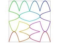
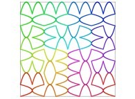
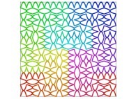
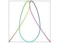
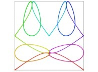
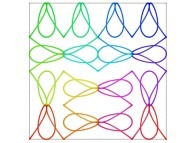
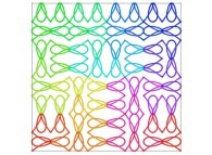
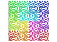
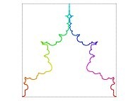
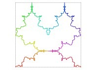
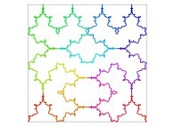
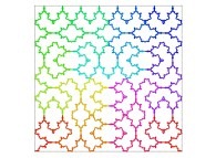
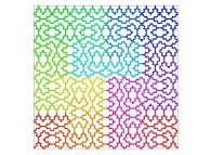
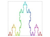
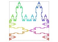
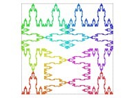
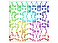
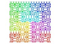
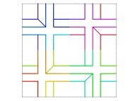
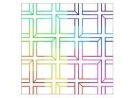
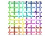
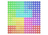
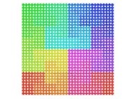
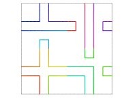
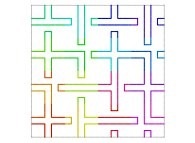

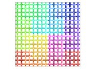
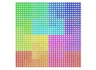
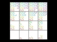
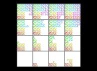
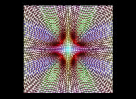
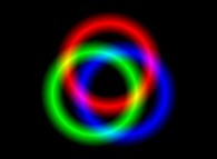
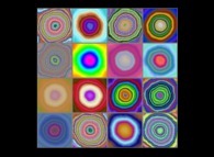
Here is the "mapping" of a few pictures by means of a bidimensional Hilbert curve:
:
 | ==>
[iteration 11] | 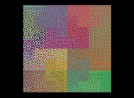 |
 | ==>
[iteration 10] | 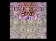 |
 | ==>
[iteration 9] | 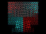 |
 | ==>
[iteration 10] | 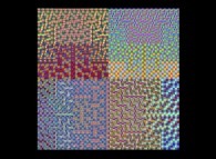 |
4-The tridimensional Hilbert Curves:
Let's C1(T) being
a parametric curve
defined by means of 3 real functions of T
(T ∈ [0,1])
X1(T) ∈ [0,1], Y1(T) ∈ [0,1] and Z1(T) ∈ [0,1]
such as
:
X1(T=0)=0 Y1(T=0)=0 Z1(T=0)=0 (lower left foreground corner)
X1(T=1)=1 Y1(T=1)=0 Z1(T=1)=0 (lower right foreground corner)
Then one defines a sequence of curves Ci(T) (i >= 1) as follows
:
Ci(T) = {Xi(T),Yi(T),Zi(T)} ∈ [0,1]x[0,1]x[0,1] --> Ci+1(T) = {Xi+1(T),Yi+1(T),Zi+1(T)} ∈ [0,1]x[0,1]x[0,1]
                    if T ∈ [0,1/8[:
                              Xi+1(T) =   Xi(8T-0)
                              Yi+1(T) =   Zi(8T-0)
                              Zi+1(T) =   Yi(8T-0)
                                                   Transformation 1
                    if T ∈ [1/8,2/8[:
                              Xi+1(T) =   Zi(8T-1)
                              Yi+1(T) = 1+Yi(8T-1)
                              Zi+1(T) =   Xi(8T-1)
                                                   Transformation 2
                    if T ∈ [2/8,3/8[:
                              Xi+1(T) = 1+Xi(8T-2)
                              Yi+1(T) = 1+Yi(8T-2)
                              Zi+1(T) =   Zi(8T-2)
                                                   Transformation 3
                    if T ∈ [3/8,4/8[:
                              Xi+1(T) = 1+Zi(8T-3)
                              Yi+1(T) = 1-Xi(8T-3)
                              Zi+1(T) = 1-Yi(8T-3)
                                                   Transformation 4
                    if T ∈ [4/8,5/8[:
                              Xi+1(T) = 2-Zi(8T-4)
                              Yi+1(T) = 1-Xi(8T-4)
                              Zi+1(T) = 1+Yi(8T-4)
                                                   Transformation 5
                    if T ∈ [5/8,6/8[:
                              Xi+1(T) = 1+Xi(8T-5)
                              Yi+1(T) = 1+Yi(8T-5)
                              Zi+1(T) = 1+Zi(8T-5)
                                                   Transformation 6
                    if T ∈ [6/8,7/8[:
                              Xi+1(T) = 1-Zi(8T-6)
                              Yi+1(T) = 1+Yi(8T-6)
                              Zi+1(T) = 2-Xi(8T-6)
                                                   Transformation 7
                    if T ∈ [7/8,1]:
                              Xi+1(T) =   Xi(8T-7)
                              Yi+1(T) = 1-Zi(8T-7)
                              Zi+1(T) = 2-Yi(8T-7)
                                                   Transformation 8
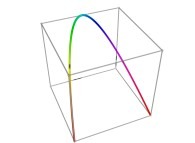
Please note that 8=2d where d=3 is the space dimension.
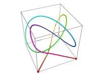
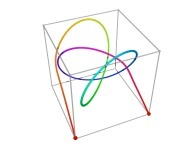
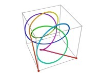
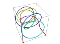
See a special C1(T) curve 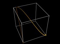 in order to understand the geometrical meaning of the 8 transformations
 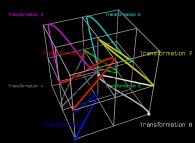 and of their order
 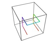 .
.
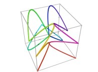
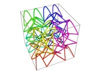
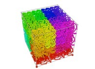
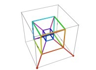
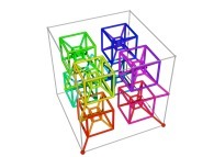
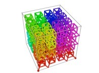
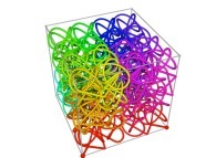
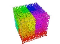
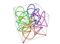
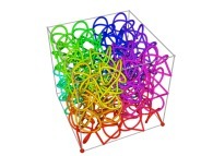
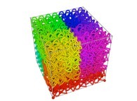
Here are the four first tridimensional Hilbert curves with an increasing number of iterations
:

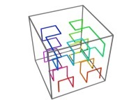
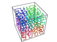
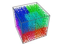 [See the used color set to display the parameter T]
See the construction of one of them
:


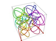
Here are some examples of Hilbert-like tridimensional curves using different generating curves and in
particular "open" knots
:


[More information about Peano Curves and Infinite Knots -in english/en anglais-]
[Plus d'informations à propos des Courbes de Peano et des Nœuds Infinis -en français/in french-]
5-Tridimensional Surfaces (Bidimensional Manifolds):
Many surfaces -bidimensional manifolds- in a tridimensional space
can be defined using a set of three equations:
X = Fx(u,v)
Y = Fy(u,v)
Z = Fz(u,v)
with:
u ∈ [Umin,Umax]
v ∈ [Vmin,Vmax]
For example:
Fx(u,v) = R.sin(u).cos(v)
Fy(u,v) = R.sin(u).sin(v)
Fz(u,v) = R.cos(u)
with:
u ∈ [0,pi]
v ∈ [0,2.pi]
defines a sphere with R as the radius and the origin of the coordinates as the center.
[Umin,Umax]*[Vmin,Vmax] then defined a bidimensional rectangular domain D.
                       v ^
                         |
                    V    |...... ---------------------------
                     max |      |+++++++++++++++++++++++++++|
                         |      |+++++++++++++++++++++++++++|
                         |      |+++++++++++++++++++++++++++|
                         |      |+++++++++++++++++++++++++++|
                         |      |+++++++++++++++++++++++++++|
                         |      |+++++++++++++++++++++++++++|
                         |      |+++++++++++++++++++++++++++|
                         |      |+++++++++++++++++++++++++++|
                         |      |+++++++++++++++++++++++++++|
                    V    |...... ---------------------------
                     min |      :                           :
                         |      :                           :
                         O------------------------------------------------->
                                U                           U              u
                                 min                         max
Let's define a curve that fills the [0,1]x[0,1] square
:
                         ^
                         |
                       1 |---------------
                         | +++++   +++++ |
                         | +   +   +   + |
                         | +   +++++   + |
                         | +           + |
                         | +++++   +++++ |
                         |     +   +     |
                         | +++++   +++++ |
                       0 O------------------------>
                         0               1
Obviously one can define a mapping between the [0,1]x[0,1] square and the [Umin,Umax]*[Vmin,Vmax] domain
:
                       v ^
                         |
                    V    |...... ---------------------------
                     max |      | ++++++++         ++++++++ |
                         |      | +      +         +      + |
                         |      | +      +         +      + |
                         |      | +      +++++++++++      + |
                         |      | +           C           + |
                         |      | ++++++++         ++++++++ |
                         |      |        +         +        |
                         |      |        +         +        |
                         |      | ++++++++         ++++++++ |
                    V    |...... ---------------------------
                     min |      :                           :
                         |      :                           :
                         O------------------------------------------------->
                                U                           U              u
                                 min                         max
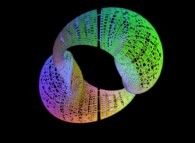
Then it suffices to display only the points {Fx(u,v),Fy(u,v),Fz(u,v)}
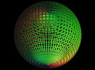
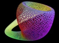
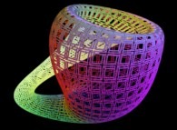
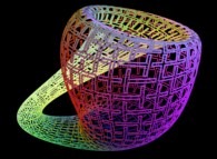
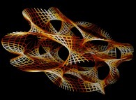
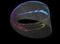
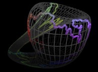
with {u,v} on the preceding curve C to fill the surface with C....
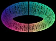
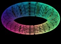
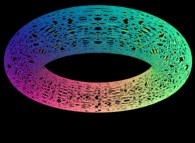
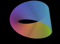
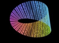
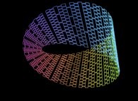
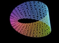
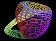
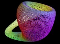
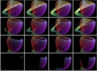
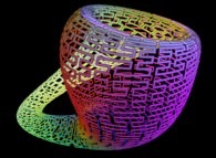
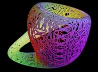
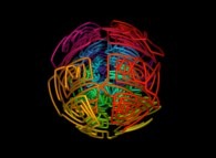
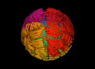
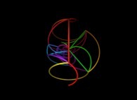
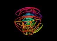
Here are some examples of this process
:
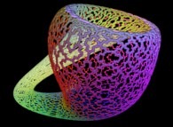
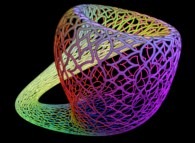
| Surface | ==> | C Curve | ==> | Surface filling Curve |
 | ==> |  | ==> |  |
 | ==> |  | ==> |  |
 | ==> |  | ==> |  |
 | ==> |  | ==> |  |
 | ==> |  | ==> |  |
 | ==> |  | ==> |  |
 | ==> |  | ==> |  |
 | ==> |  | ==> |  |
 | ==> |  | ==> |  |
6-Tridimensional Manifolds:
Many tridimensional manifolds in a tridimensional space
can be defined using a set of three equations:
X = Fx(u,v,w)
Y = Fy(u,v,w)
Z = Fz(u,v,w)
with:
u ∈ [Umin,Umax]
v ∈ [Vmin,Vmax]
w ∈ [Wmin,Wmax]
[Umin,Umax]*[Vmin,Vmax]*[Wmin,Wmax] then defined a tridimensional rectangular domain D.
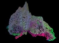
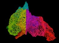
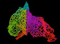
It is obvious to generalize the preceding bidimensional process in the tridimensional space...
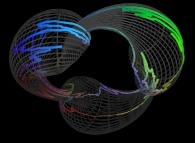
Here are some examples of this process
:
| Tridimensional Manifold | ==> | C Curve | ==> | Tridimensional Manifold filling Curve |
7-Beyond:
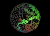
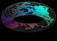
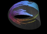
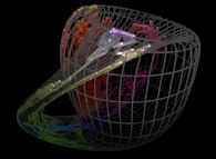
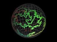
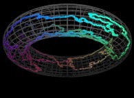
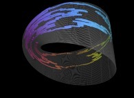
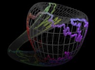
Instead of using space-filling curves in order to fill the {u,v} and {u,v,w} bi- and tridimensional domains,
obviously one can use any means available and, for example, the bi-
and the tridimensional brownian motions respectively....
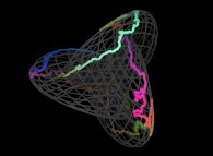
Here are some examples of these extended processes
:


Copyright © Jean-François COLONNA, 2023-2025.
Copyright © CMAP (Centre de Mathématiques APpliquées) UMR CNRS 7641 / École polytechnique, Institut Polytechnique de Paris, 2023-2025.


 [See the used color set to display the parameter T]


 [See the used color set to display the parameter T]
 in order to understand the geometrical meaning of the 4 transformations
  and of their order
  .
.


 [See the used color set to display the parameter T]


 in order to understand the geometrical meaning of the 8 transformations
  and of their order
  .
.


 [See the used color set to display the parameter T]
