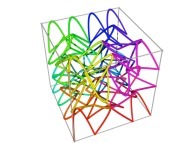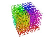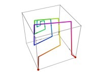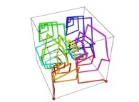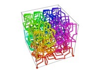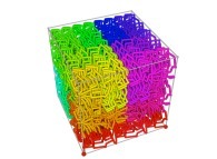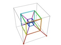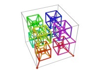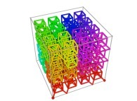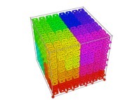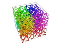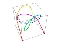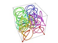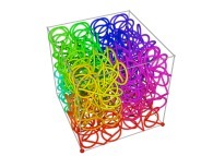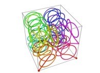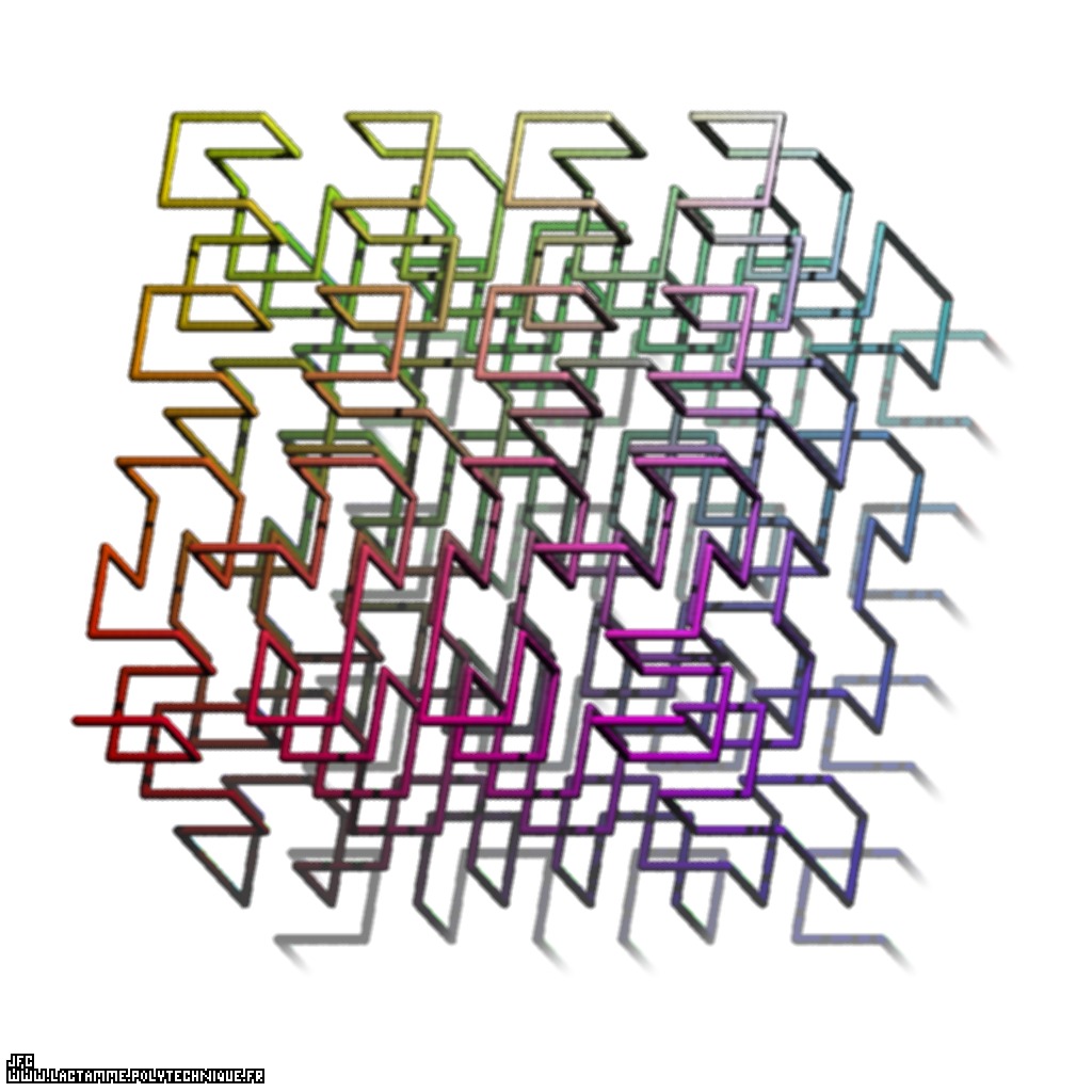
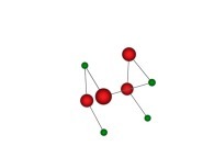
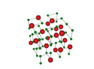
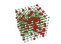
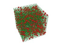
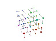
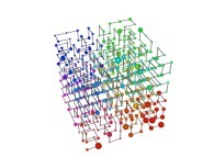
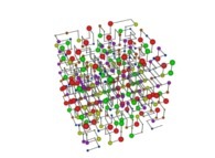
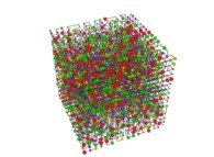
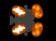
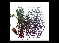
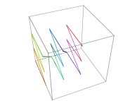
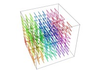
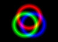
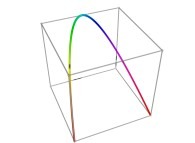
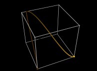
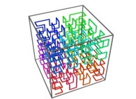
Tridimensional Hilbert Curve -iteration 3- [Courbe de Hilbert tridimensionnelle -itération 3-].
Tridimensional Hilbert Curve -iteration 3- [Courbe de Hilbert tridimensionnelle -itération 3-].
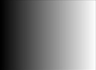
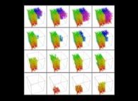
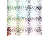
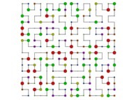
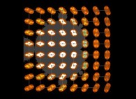
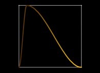
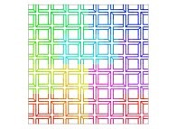
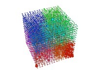 See the used color set to display the parameter T.
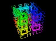
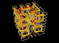
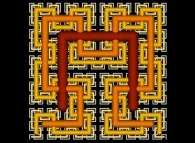
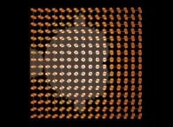
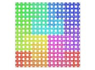
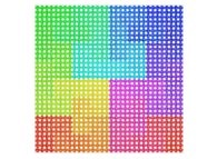
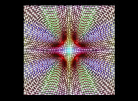
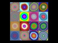
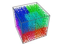
 See the used color set to display the pi digits.
 See the used color set to display the parameter T.
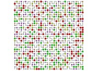 See the used color set to display the pi digits.
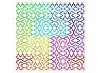
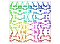
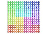
[0,1] --> [0,1]x[0,1]Let's T being a real number defined using the base 3 :
T = 0.A1A2A3... ∈ [0,1] with Ai ∈ {0,1,2}
Let's X(T) and Y(T) being two real functions of T defined as
:
X(T) = 0.B1B2B3... ∈ [0,1] with Bi ∈ {0,1,2}
Y(T) = 0.C1C2C3... ∈ [0,1] with Ci ∈ {0,1,2}
with
:
Bn = A2n-1 if A2+A4+...+A2n-0 is even
Bn = 2-A2n-1 otherwise
Cn = A2n if A1+A3+...+A2n-1 is even
Cn = 2-A2n otherwise
 [See the used color set to display the parameter T]
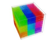
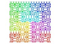
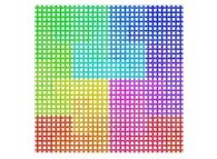
[0,1] --> [0,1]x[0,1]x[0,1]as a generalization of the bidimensional one.
T = 0.A1A2A3... ∈ [0,1] with Ai ∈ {0,1,2}
Let's X(T), Y(T) and Z(T) being three real functions of T defined as:
X(T) = 0.B1B2B3... ∈ [0,1] with Bi ∈ {0,1,2}
Y(T) = 0.C1C2C3... ∈ [0,1] with Ci ∈ {0,1,2}
Y(T) = 0.D1D2D3... ∈ [0,1] with Di ∈ {0,1,2}
with
:
Bn = A3n-2 if A3+A6+...+A3n-0 is even
Bn = 2-A3n-2 otherwise
Cn = A3n-1 if A2+A5+...+A3n-1 is even
Cn = 2-A3n-1 otherwise
Dn = A3n if A1+A4+...+A3n-2 is even
Dn = 2-A3n otherwise
 [See the used color set to display the parameter T]
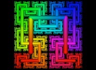
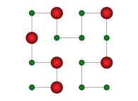
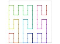
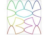
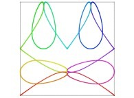
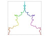
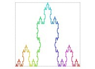
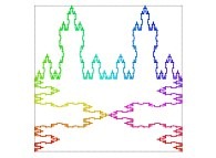
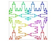
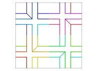
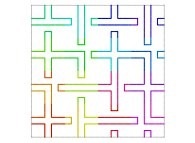
 defined by means of 2 real functions of T
(T ∈ [0,1])
X1(T) ∈ [0,1] and Y1(T) ∈ [0,1]
such as
:
defined by means of 2 real functions of T
(T ∈ [0,1])
X1(T) ∈ [0,1] and Y1(T) ∈ [0,1]
such as
:
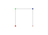
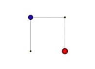
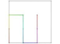
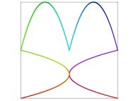
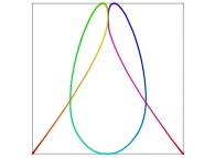
X1(T=0)=0 Y1(T=0)=0 (lower left corner)
X1(T=1)=1 Y1(T=1)=0 (lower right corner)
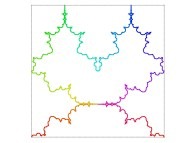
Ci(T) = {Xi(T),Yi(T)} ∈ [0,1]x[0,1] --> Ci+1(T) = {Xi+1(T),Yi+1(T)} ∈ [0,1]x[0,1]
                    if T ∈ [0,1/4[:
                              Xi+1(T) =   Yi(4T-0)
                              Yi+1(T) =   Xi(4T-0)
                                                   Transformation 1
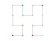
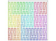
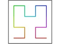
                    if T ∈ [1/4,2/4[:
                              Xi+1(T) =   Xi(4T-1)
                              Yi+1(T) = 1+Yi(4T-1)
                                                   Transformation 2
                    if T ∈ [2/4,3/4[:
                              Xi+1(T) = 1+Xi(4T-2)
                              Yi+1(T) = 1+Yi(4T-2)
                                                   Transformation 3
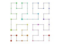
                    if T ∈ [3/4,1]:
                              Xi+1(T) = 2-Yi(4T-3)
                              Yi+1(T) = 1-Xi(4T-3)
                                                   Transformation 4
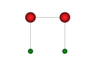
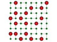
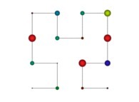
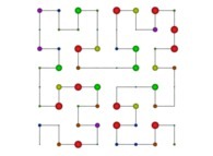
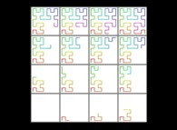
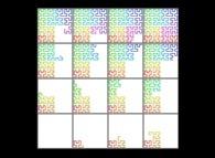
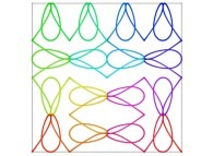
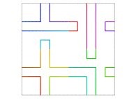
 in order to understand the geometrical meaning of the 4 transformations
 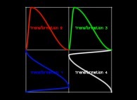 and of their order
 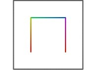 .
.
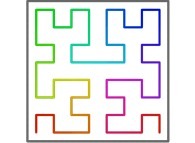
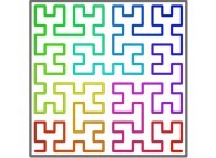
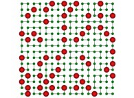
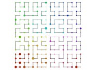
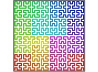 [See the used color set to display the parameter T]
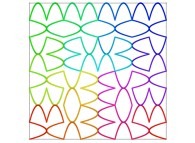
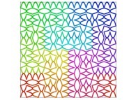
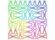
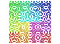
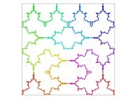
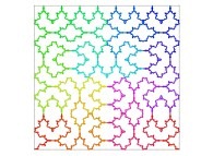
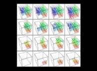
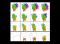
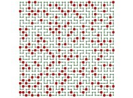
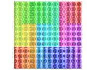
 | ==> [iteration 11] | 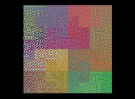 |
 | ==> [iteration 10] | 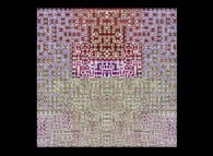 |
 | ==> [iteration 9] | 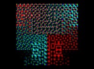 |
 | ==> [iteration 10] | 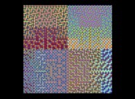 |
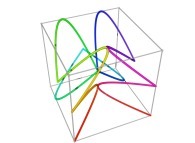
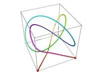
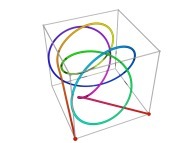
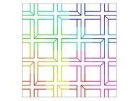
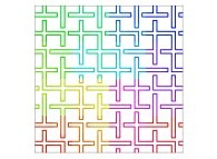
 defined by means of 3 real functions of T
(T ∈ [0,1])
X1(T) ∈ [0,1], Y1(T) ∈ [0,1] and Z1(T) ∈ [0,1]
such as
:
defined by means of 3 real functions of T
(T ∈ [0,1])
X1(T) ∈ [0,1], Y1(T) ∈ [0,1] and Z1(T) ∈ [0,1]
such as
:
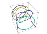
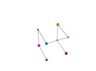
X1(T=0)=0 Y1(T=0)=0 Z1(T=0)=0 (lower left foreground corner)
X1(T=1)=1 Y1(T=1)=0 Z1(T=1)=0 (lower right foreground corner)
Ci(T) = {Xi(T),Yi(T),Zi(T)} ∈ [0,1]x[0,1]x[0,1] --> Ci+1(T) = {Xi+1(T),Yi+1(T),Zi+1(T)} ∈ [0,1]x[0,1]x[0,1]
                    if T ∈ [0,1/8[:
                              Xi+1(T) =   Xi(8T-0)
                              Yi+1(T) =   Zi(8T-0)
                              Zi+1(T) =   Yi(8T-0)
                                                   Transformation 1
                    if T ∈ [1/8,2/8[:
                              Xi+1(T) =   Zi(8T-1)
                              Yi+1(T) = 1+Yi(8T-1)
                              Zi+1(T) =   Xi(8T-1)
                                                   Transformation 2
                    if T ∈ [2/8,3/8[:
                              Xi+1(T) = 1+Xi(8T-2)
                              Yi+1(T) = 1+Yi(8T-2)
                              Zi+1(T) =   Zi(8T-2)
                                                   Transformation 3
                    if T ∈ [3/8,4/8[:
                              Xi+1(T) = 1+Zi(8T-3)
                              Yi+1(T) = 1-Xi(8T-3)
                              Zi+1(T) = 1-Yi(8T-3)
                                                   Transformation 4
                    if T ∈ [4/8,5/8[:
                              Xi+1(T) = 2-Zi(8T-4)
                              Yi+1(T) = 1-Xi(8T-4)
                              Zi+1(T) = 1+Yi(8T-4)
                                                   Transformation 5
                    if T ∈ [5/8,6/8[:
                              Xi+1(T) = 1+Xi(8T-5)
                              Yi+1(T) = 1+Yi(8T-5)
                              Zi+1(T) = 1+Zi(8T-5)
                                                   Transformation 6
                    if T ∈ [6/8,7/8[:
                              Xi+1(T) = 1-Zi(8T-6)
                              Yi+1(T) = 1+Yi(8T-6)
                              Zi+1(T) = 2-Xi(8T-6)
                                                   Transformation 7
                    if T ∈ [7/8,1]:
                              Xi+1(T) =   Xi(8T-7)
                              Yi+1(T) = 1-Zi(8T-7)
                              Zi+1(T) = 2-Yi(8T-7)
                                                   Transformation 8
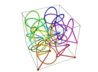
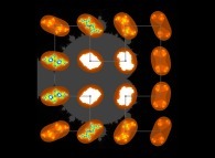
 in order to understand the geometrical meaning of the 8 transformations
 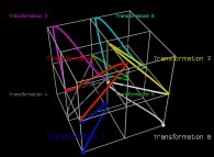 and of their order
 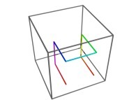 .
.
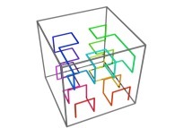
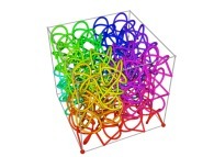
 [See the used color set to display the parameter T]